Deep SORT 是多目标跟踪 (Multi-Object Tracking) 中常用到的一种算法,是一个 Detection Based Tracking 的方法。这个算法工业界关注度非常高,在知乎上有很多文章都是使用了 Deep SORT 进行工程部署。笔者将参考前辈的博客,结合自己的实践 (理论 & 代码) 对 Deep SORT 算法进行代码层面的解析。
在之前笔者写的一篇 Deep SORT 论文阅读总结中,总结了 DeepSORT 论文中提到的核心观点,如果对 Deep SORT 不是很熟悉,可以先理解一下,然后再来看解读代码的部分。
由于知乎对文章篇幅有限制,所以分上下篇发。
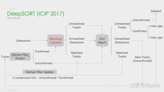
上篇将梳理 SORT、Deep SORT,以类图为主,讲解 DeepSORT 代码部分的各个模块。
下篇主要是梳理运行的流程,对照流程图进行代码层面理解。以及最后的总结 + 代码推荐。
1. MOT 主要步骤
在《DEEP LEARNING IN VIDEO MULTI-OBJECT TRACKING: A SURVEY》这篇基于深度学习的多目标跟踪的综述中,描述了 MOT 问题中四个主要步骤:
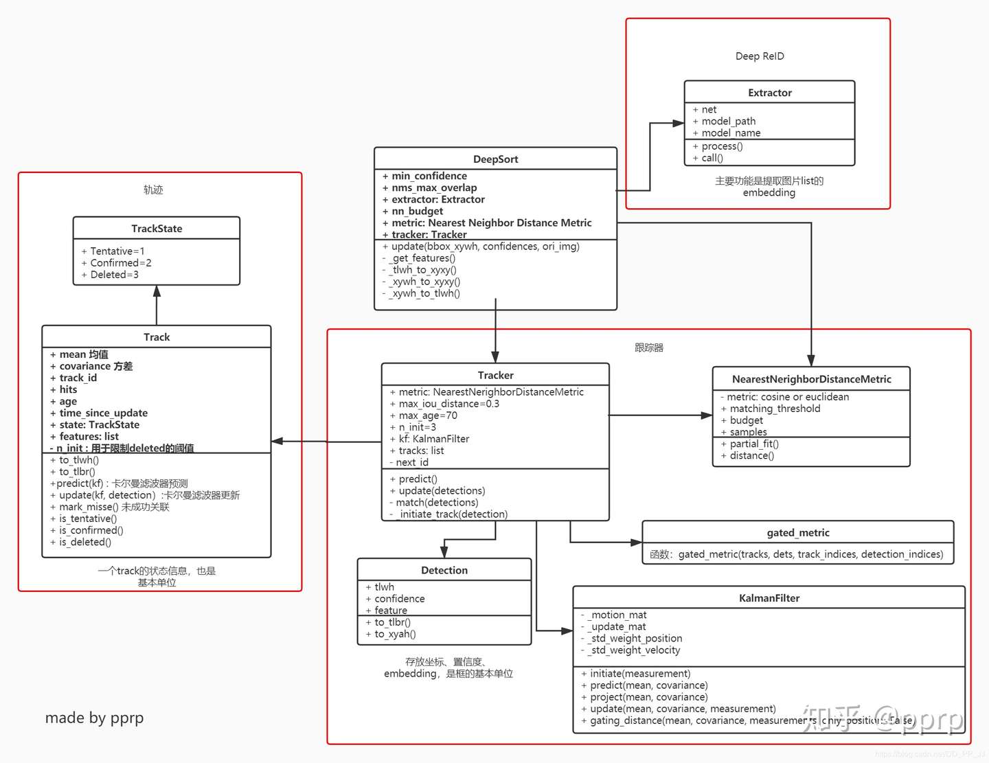
classDetection(object): """ This class represents a bounding box detection in a single image. """ def__init__(self, tlwh, confidence, feature): self.tlwh = np.asarray(tlwh, dtype=np.float) self.confidence = float(confidence) self.feature = np.asarray(feature, dtype=np.float32) defto_tlbr(self): """Convert bounding box to format `(min x, min y, max x, max y)`, i.e., `(top left, bottom right)`. """ ret = self.tlwh.copy() ret[2:] += ret[:2] return ret defto_xyah(self): """Convert bounding box to format `(center x, center y, aspect ratio, height)`, where the aspect ratio is `width / height`. """ ret = self.tlwh.copy() ret[:2] += ret[2:] / 2 ret[2] /= ret[3] return ret
Detection 类用于保存通过目标检测器得到的一个检测框,包含 top left 坐标 + 框的宽和高,以及该 bbox 的置信度还有通过 reid 获取得到的对应的 embedding。除此以外提供了不同 bbox 位置格式的转换方法:
classTrack: # 一个轨迹的信息,包含(x,y,a,h) & v """ A single target track with state space `(x, y, a, h)` and associated velocities, where `(x, y)` is the center of the bounding box, `a` is the aspect ratio and `h` is the height. """
def_preprocess(self, im_crops): """ TODO: 1. to float with scale from 0 to 1 2. resize to (64, 128) as Market1501 dataset did 3. concatenate to a numpy array 3. to torch Tensor 4. normalize """ def_resize(im, size): return cv2.resize(im.astype(np.float32) / 255., size)
im_batch = torch.cat([ self.norm(_resize(im, self.size)).unsqueeze(0) for im in im_crops ],dim=0).float() return im_batch
def__call__(self, im_crops): im_batch = self._preprocess(im_crops) with torch.no_grad(): im_batch = im_batch.to(self.device) features = self.net(im_batch) return features.cpu().numpy()
模型训练是按照传统 ReID 的方法进行,使用 Extractor 类的时候输入为一个 list 的图片,得到图片对应的特征。
classTracker: # 是一个多目标tracker,保存了很多个track轨迹 # 负责调用卡尔曼滤波来预测track的新状态+进行匹配工作+初始化第一帧 # Tracker调用update或predict的时候,其中的每个track也会各自调用自己的update或predict """ This is the multi-target tracker. """
self.kf = kalman_filter.KalmanFilter()# 卡尔曼滤波器 self.tracks = [] # 保存一系列轨迹 self._next_id = 1# 下一个分配的轨迹id defpredict(self): # 遍历每个track都进行一次预测 """Propagate track state distributions one time step forward. This function should be called once every time step, before `update`. """ for track in self.tracks: track.predict(self.kf)
defupdate(self, detections): # 进行测量的更新和轨迹管理 """Perform measurement update and track management. Parameters ---------- detections : List[deep_sort.detection.Detection] A list of detections at the current time step. """ # Run matching cascade. matches, unmatched_tracks, unmatched_detections = \ self._match(detections)
# Update track set. # 1. 针对匹配上的结果 for track_idx, detection_idx in matches: # track更新对应的detection self.tracks[track_idx].update(self.kf, detections[detection_idx])
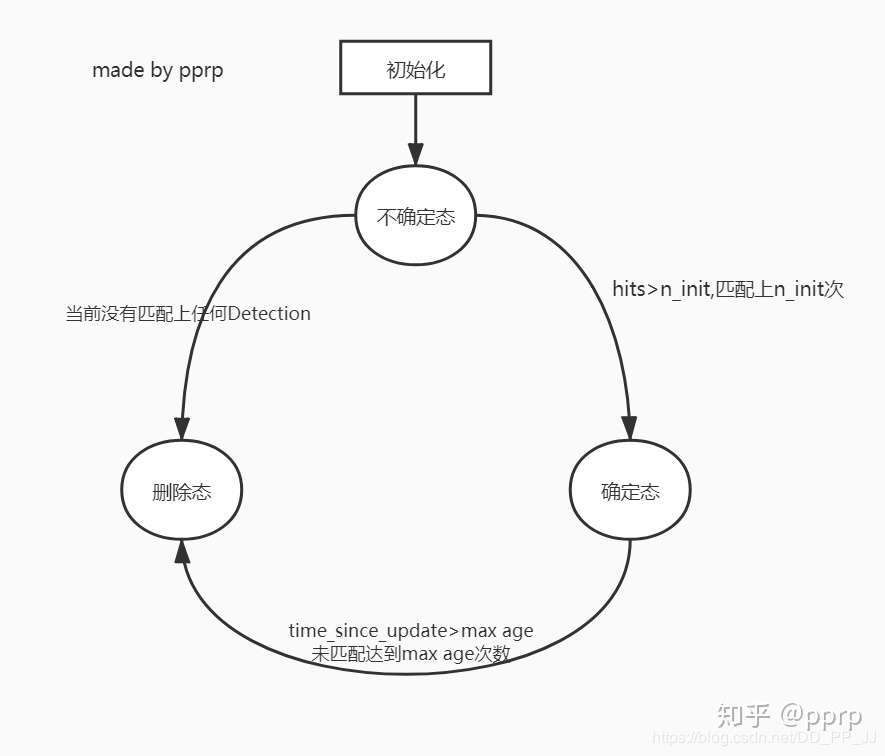
# 2. 针对未匹配的tracker,调用mark_missed标记 # track失配,若待定则删除,若update时间很久也删除 # max age是一个存活期限,默认为70帧 for track_idx in unmatched_tracks: self.tracks[track_idx].mark_missed()
# 3. 针对未匹配的detection, detection失配,进行初始化 for detection_idx in unmatched_detections: self._initiate_track(detections[detection_idx])
# 得到最新的tracks列表,保存的是标记为confirmed和Tentative的track self.tracks = [t for t in self.tracks ifnot t.is_deleted()]
# Update distance metric. active_targets = [t.track_id for t in self.tracks if t.is_confirmed()] # 获取所有confirmed状态的track id features, targets = [], [] for track in self.tracks: ifnot track.is_confirmed(): continue features += track.features # 将tracks列表拼接到features列表 # 获取每个feature对应的track id targets += [track.track_id for _ in track.features] track.features = []
# Split track set into confirmed and unconfirmed tracks. # 划分不同轨迹的状态 confirmed_tracks = [ i for i, t inenumerate(self.tracks) if t.is_confirmed() ] unconfirmed_tracks = [ i for i, t inenumerate(self.tracks) ifnot t.is_confirmed() ]
# 将所有状态为未确定态的轨迹和刚刚没有匹配上的轨迹组合为iou_track_candidates, # 进行IoU的匹配 iou_track_candidates = unconfirmed_tracks + [ k for k in unmatched_tracks_a if self.tracks[k].time_since_update == 1# 刚刚没有匹配上 ] # 未匹配 unmatched_tracks_a = [ k for k in unmatched_tracks_a if self.tracks[k].time_since_update != 1# 已经很久没有匹配上 ]
# 1. 分配track_indices和detection_indices if track_indices isNone: track_indices = list(range(len(tracks)))
if detection_indices isNone: detection_indices = list(range(len(detections)))
unmatched_detections = detection_indices
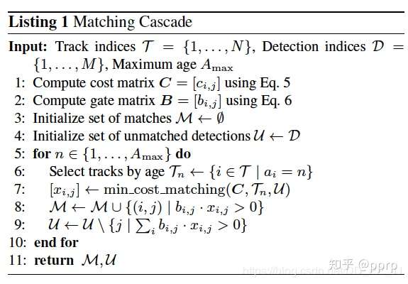
matches = [] # cascade depth = max age 默认为70 for level inrange(cascade_depth): iflen(unmatched_detections) == 0: # No detections left break
track_indices_l = [ k for k in track_indices if tracks[k].time_since_update == 1 + level ] iflen(track_indices_l) == 0: # Nothing to match at this level continue
detections = [ Detection(bbox_tlwh[i], conf, features[i]) for i, conf inenumerate(confidences) if conf > self.min_confidence ] # 筛选小于min_confidence的目标,并构造一个Detection对象构成的列表 # Detection是一个存储图中一个bbox结果 # 需要:1. bbox(tlwh形式) 2. 对应置信度 3. 对应embedding
# run on non-maximum supression boxes = np.array([d.tlwh for d in detections]) scores = np.array([d.confidence for d in detections])
# 使用非极大抑制 # 默认nms_thres=1的时候开启也没有用,实际上并没有进行非极大抑制 indices = non_max_suppression(boxes, self.nms_max_overlap, scores) detections = [detections[i] for i in indices]
defpredict(self): # 遍历每个track都进行一次预测 """Propagate track state distributions one time step forward. This function should be called once every time step, before `update`. """ for track in self.tracks: track.predict(self.kf)
defupdate(self, detections): # 进行测量的更新和轨迹管理 """Perform measurement update and track management. Parameters ---------- detections : List[deep_sort.detection.Detection] A list of detections at the current time step. """ # Run matching cascade. matches, unmatched_tracks, unmatched_detections = \ self._match(detections)
# Update track set. # 1. 针对匹配上的结果 for track_idx, detection_idx in matches: # track更新对应的detection self.tracks[track_idx].update(self.kf, detections[detection_idx])
# 2. 针对未匹配的tracker,调用mark_missed标记 # track失配,若待定则删除,若update时间很久也删除 # max age是一个存活期限,默认为70帧 for track_idx in unmatched_tracks: self.tracks[track_idx].mark_missed()
# 3. 针对未匹配的detection, detection失配,进行初始化 for detection_idx in unmatched_detections: self._initiate_track(detections[detection_idx])
# 得到最新的tracks列表,保存的是标记为confirmed和Tentative的track self.tracks = [t for t in self.tracks ifnot t.is_deleted()]
# Update distance metric. active_targets = [t.track_id for t in self.tracks if t.is_confirmed()] # 获取所有confirmed状态的track id features, targets = [], [] for track in self.tracks: ifnot track.is_confirmed(): continue features += track.features # 将tracks列表拼接到features列表 # 获取每个feature对应的track id targets += [track.track_id for _ in track.features] track.features = []
# Split track set into confirmed and unconfirmed tracks. # 划分不同轨迹的状态 confirmed_tracks = [ i for i, t inenumerate(self.tracks) if t.is_confirmed() ] unconfirmed_tracks = [ i for i, t inenumerate(self.tracks) ifnot t.is_confirmed() ]
# 将所有状态为未确定态的轨迹和刚刚没有匹配上的轨迹组合为iou_track_candidates, # 进行IoU的匹配 iou_track_candidates = unconfirmed_tracks + [ k for k in unmatched_tracks_a if self.tracks[k].time_since_update == 1# 刚刚没有匹配上 ] # 未匹配 unmatched_tracks_a = [ k for k in unmatched_tracks_a if self.tracks[k].time_since_update != 1# 已经很久没有匹配上 ]
# 1. 分配track_indices和detection_indices if track_indices isNone: track_indices = list(range(len(tracks)))
if detection_indices isNone: detection_indices = list(range(len(detections)))
unmatched_detections = detection_indices
matches = [] # cascade depth = max age 默认为70 for level inrange(cascade_depth): iflen(unmatched_detections) == 0: # No detections left break
track_indices_l = [ k for k in track_indices if tracks[k].time_since_update == 1 + level ] iflen(track_indices_l) == 0: # Nothing to match at this level continue
# 这几个for循环用于对匹配结果进行筛选,得到匹配和未匹配的结果 for col, detection_idx inenumerate(detection_indices): if col notin col_indices: unmatched_detections.append(detection_idx)
for row, track_idx inenumerate(track_indices): if row notin row_indices: unmatched_tracks.append(track_idx)
for row, col inzip(row_indices, col_indices): track_idx = track_indices[row] detection_idx = detection_indices[col] if cost_matrix[row, col] > max_distance: unmatched_tracks.append(track_idx) unmatched_detections.append(detection_idx) else: matches.append((track_idx, detection_idx)) # 得到匹配,未匹配轨迹,未匹配检测 return matches, unmatched_tracks, unmatched_detections
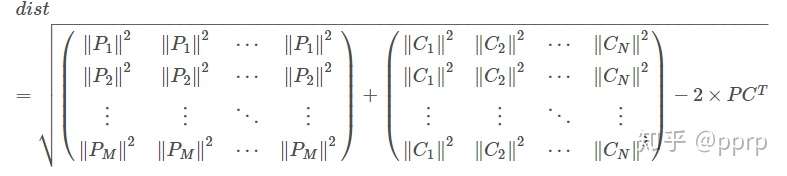
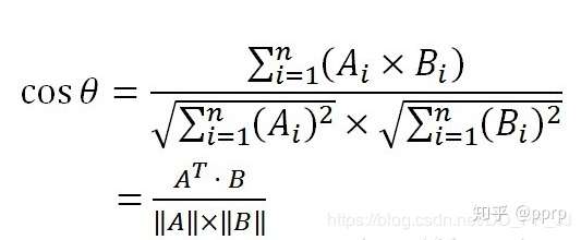
defgated_metric(tracks, dets, track_indices, detection_indices): # 功能: 用于计算track和detection之间的距离,代价函数 # 需要使用在KM算法之前 # 调用: # cost_matrix = distance_metric(tracks, detections, # track_indices, detection_indices) features = np.array([dets[i].feature for i in detection_indices]) targets = np.array([tracks[i].track_id for i in track_indices])
次,该目标 ID 将从图片中删除。