【精华】模型部署实例（OpenVINO、TensorRT）

文章目录

（1）OpenVINO 部署 NanoDet 模型
（2）TensorRT 部署深度学习模型

（1）OpenVINO 部署 NanoDet 模型

1> nanodet 简介

NanoDet （https://github.com/RangiLyu/nanodet）是一个速度超快和轻量级的 Anchor-free 目标检测模型。想了解算法本身的可以去搜一搜之前机器之心的介绍。

2> 环境配置

Ubuntu：18.04
OpenVINO：2020.4
OpenCV：3.4.2
OpenVINO 和 OpenCV 安装包（编译好了，也可以自己从官网下载自己编译）可以从链接: https://pan.baidu.com/s/1zxtPKm-Q48Is5mzKbjGHeg 密码: gw5c 下载
OpenVINO 安装

tar -xvzf l_openvino_toolkit_p_2020.4.287.tgz

cd l_openvino_toolkit_p_2020.4.287
sudo ./install_GUI.sh 一路next安装

cd /opt/intel/openvino/install_dependencies
sudo ./install_openvino_dependencies.sh

vi ~/.bashrc

把如下两行放置到 bashrc 文件尾

1 2	source /opt/intel/openvino/bin/setupvars.sh source /opt/intel/openvino/opencv/setupvars.sh

source ~/.bashrc 激活环境
模型优化配置步骤

1 2	cd /opt/intel/openvino/deployment_tools/model_optimizer/install_prerequisites sudo ./install_prerequisites_onnx.sh（模型是从onnx转为IR文件，只需配置onnx依赖）

OpenCV 配置

1	tar -xvzf opencv-3.4.2.zip # 解压OpenCV到用户根目录即可，以便后续调用。（这是我编译好的版本，有需要可以自己编译）

3> NanoDet 模型训练和转换 ONNX

git clone https://github.com/Wulingtian/nanodet.git
cd nanodet
cd config 配置模型文件，训练模型
定位到 nanodet 目录，进入 tools 目录，打开 export.py 文件，配置 cfg_path model_path out_path 三个参数
定位到 nanodet 目录，运行 python tools/export.py 得到转换后的 onnx 模型
python /opt/intel/openvino/deployment_tools/model_optimizer/mo_onnx.py --input_model onnx 模型 --output_dir 期望模型输出的路径。得到 IR 文件

4> NanoDet 模型部署

sudo apt install cmake 安装 cmake
git clone https://github.com/Wulingtian/nanodet_openvino.git （求 star！）
cd nanodet_openvino 打开 CMakeLists.txt 文件，修改 OpenCV_INCLUDE_DIRS 和 OpenCV_LIBS_DIR，之前已经把 OpenCV 解压到根目录了，所以按照你自己的路径指定
定位到 nanodet_openvino，cd models 把之前生成的 IR 模型（包括 bin 和 xml 文件）文件放到该目录下
定位到 nanodet_openvino， cd test_imgs 把需要测试的图片放到该目录下
定位到 nanodet_openvino，编辑 main.cpp，xml_path 参数修改为 "…/models/ 你的模型名称.xml"
编辑 num_class 设置类别数，例如：我训练的模型是安全帽检测，只有 1 类，那么设置为 1
编辑 src 设置测试图片路径，src 参数修改为 "…/test_imgs/ 你的测试图片"
定位到 nanodet_openvino
mkdir build; cd build; cmake … ;make
./detect_test 输出平均推理时间，以及保存预测图片到当前目录下，至此，部署完成！

5> 核心代码一览

//主要对图片进行预处理，包括resize和归一化
std::vector<float> Detector::prepareImage(cv::Mat &src_img){
 
    std::vector<float> result(INPUT_W * INPUT_H * 3);
    float *data = result.data();
    float ratio = float(INPUT_W) / float(src_img.cols) < float(INPUT_H) / float(src_img.rows) ? float(INPUT_W) / float(src_img.cols) : float(INPUT_H) / float(src_img.rows);
    cv::Mat flt_img = cv::Mat::zeros(cv::Size(INPUT_W, INPUT_H), CV_8UC3);
    cv::Mat rsz_img = cv::Mat::zeros(cv::Size(src_img.cols*ratio, src_img.rows*ratio), CV_8UC3);
    cv::resize(src_img, rsz_img, cv::Size(), ratio, ratio);
 
    rsz_img.copyTo(flt_img(cv::Rect(0, 0, rsz_img.cols, rsz_img.rows)));
    flt_img.convertTo(flt_img, CV_32FC3);
 
    int channelLength = INPUT_W * INPUT_H;
    std::vector<cv::Mat> split_img = {
            cv::Mat(INPUT_W, INPUT_H, CV_32FC1, data + channelLength * 2),
            cv::Mat(INPUT_W, INPUT_H, CV_32FC1, data + channelLength),
            cv::Mat(INPUT_W, INPUT_H, CV_32FC1, data)
    };
 
    cv::split(flt_img, split_img);
    for (int i = 0; i < 3; i++) {
 
        split_img[i] = (split_img[i] - img_mean[i]) / img_std[i];
    }
 
    return result;
}
 
//加载IR模型，初始化网络
bool Detector::init(string xml_path,double cof_threshold,double nms_area_threshold,int input_w, int input_h, int num_class, int r_rows, int r_cols, std::vector<int> s, std::vector<float> i_mean,std::vector<float> i_std){
    _xml_path = xml_path;
    _cof_threshold = cof_threshold;
    _nms_area_threshold = nms_area_threshold;
    INPUT_W = input_w;
    INPUT_H = input_h;
    NUM_CLASS = num_class;
    refer_rows = r_rows;
    refer_cols = r_cols;
    strides = s;
    img_mean = i_mean;
    img_std = i_std;
    Core ie;
    auto cnnNetwork = ie.ReadNetwork(_xml_path); 
 
    InputsDataMap inputInfo(cnnNetwork.getInputsInfo());
    InputInfo::Ptr& input = inputInfo.begin()->second;
    _input_name = inputInfo.begin()->first;
    input->setPrecision(Precision::FP32);
    input->getInputData()->setLayout(Layout::NCHW);
    ICNNNetwork::InputShapes inputShapes = cnnNetwork.getInputShapes();
    SizeVector& inSizeVector = inputShapes.begin()->second;
    cnnNetwork.reshape(inputShapes);
    _outputinfo = OutputsDataMap(cnnNetwork.getOutputsInfo());
    for (auto &output : _outputinfo) {
        output.second->setPrecision(Precision::FP32);
    }
    _network =  ie.LoadNetwork(cnnNetwork, "CPU");
    return true;
}
//模型推理及获取输出结果
vector<Detector::Bbox> Detector::process_frame(Mat& inframe){
 
    cv::Mat showImage = inframe.clone();
    std::vector<float> pr_img = prepareImage(inframe);
    InferRequest::Ptr infer_request = _network.CreateInferRequestPtr();
    Blob::Ptr frameBlob = infer_request->GetBlob(_input_name);
    InferenceEngine::LockedMemory<void> blobMapped = InferenceEngine::as<InferenceEngine::MemoryBlob>(frameBlob)->wmap();
    float* blob_data = blobMapped.as<float*>();
 
    memcpy(blob_data, pr_img.data(), 3 * INPUT_H * INPUT_W * sizeof(float));
 
    infer_request->Infer();
    vector<Rect> origin_rect;
    vector<float> origin_rect_cof;
    int i=0;
    vector<Bbox> bboxes;
    for (auto &output : _outputinfo) {
        auto output_name = output.first;
        Blob::Ptr blob = infer_request->GetBlob(output_name);
        LockedMemory<const void> blobMapped = as<MemoryBlob>(blob)->rmap();
        float *output_blob = blobMapped.as<float *>();
        bboxes = postProcess(showImage,output_blob);
        ++i;
    }
    return bboxes;
}
//对模型输出结果进行解码及nms
std::vector<Detector::Bbox> Detector::postProcess(const cv::Mat &src_img,
                              float *output) {
    GenerateReferMatrix();
    std::vector<Detector::Bbox> result;
    float *out = output;
    float ratio = std::max(float(src_img.cols) / float(INPUT_W), float(src_img.rows) / float(INPUT_H));
    cv::Mat result_matrix = cv::Mat(refer_rows, NUM_CLASS + 4, CV_32FC1, out);
    for (int row_num = 0; row_num < refer_rows; row_num++) {
        Detector::Bbox box;
        auto *row = result_matrix.ptr<float>(row_num);
        auto max_pos = std::max_element(row + 4, row + NUM_CLASS + 4);
        box.prob = row[max_pos - row];
        if (box.prob < _cof_threshold)
            continue;
        box.classes = max_pos - row - 4;
        auto *anchor = refer_matrix.ptr<float>(row_num);
        box.x = (anchor[0] - row[0] * anchor[2] + anchor[0] + row[2] * anchor[2]) / 2 * ratio;
        box.y = (anchor[1] - row[1] * anchor[2] + anchor[1] + row[3] * anchor[2]) / 2 * ratio;
        box.w = (row[2] + row[0]) * anchor[2] * ratio;
        box.h = (row[3] + row[1]) * anchor[2] * ratio;
        result.push_back(box);
    }
    NmsDetect(result);
    return result;
}

6> 推理时间展示及预测结果展示

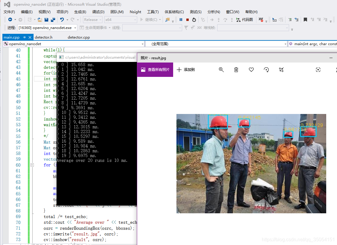
我的老笔记本平均推理时间 15ms 左右，CPU 下实时推理

安全帽检测结果

至此完成了 NanoDet 在 X86 CPU 上的部署，希望有帮助到大家。

（2）TensorRT 部署深度学习模型

原帖：https://zhuanlan.zhihu.com/p/84125533

1> 背景

目前主流的深度学习框架（caffe，mxnet，tensorflow，pytorch 等）进行模型推断的速度都并不优秀，在实际工程中用上述的框架进行模型部署往往是比较低效的。而通过 Nvidia 推出的 tensorRT 工具来部署主流框架上训练的模型能够极大的提高模型推断的速度，往往相比与原本的框架能够有至少 1 倍以上的速度提升，同时占用的设备内存也会更加的少。因此对是所有需要部署模型的同志来说，掌握用 tensorRT 来部署深度学习模型的方法是非常有用的。

2> 相关技术

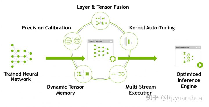
上面的图片取自 TensorRT 的官网，里面列出了 tensorRT 使用的一些技术。可以看到比较成熟的深度学习落地技术：模型量化、动态内存优化、层的融合等技术均已经在 tensorRT 中集成了，这也是它能够极大提高模型推断速度的原因。总体来说 tensorRT 将训练好的模型通过一系列的优化技术转化为了能够在特定平台（GPU）上以高性能运行的代码，也就是最后图中生成的 Inference engine。目前也有一些其他的工具能够实现类似 tensorRT 的功能，例如 TVM，TensorComprehensions 也能有效的提高模型在特定平台上的推断速度，但是由于目前企业主流使用的都是 Nvidia 生产的计算设备，在这些设备上 nvidia 推出的 tensorRT 性能相比其他工具会更有优势一些。而且 tensorRT 依赖的代码库仅仅包括 C++ 和 cuda，相对与其他工具要更为精简一些。

3> tensorflow 模型 tensorRT 部署教程

实际工程部署中多采用 c 进行部署，因此在本教程中也使用的是 tensorRT 的 CAPI，tensorRT 版本为 5.1.5。具体 tensorRT 安装可参考教程 [深度学习] TensorRT 安装，以及官网的安装说明。

（1）模型持久化

部署 tensorflow 模型的第一步是模型持久化，将模型结构和权重保存到一个.pb 文件当中。

1
2
3

pb_graph = tf.graph_util.convert_variables_to_constants(sess, sess.graph.as_graph_def(), [v.op.name for v in outputs])
with tf.gfile.FastGFile('./pbmodel_name.pb', mode='wb') as f:
    f.write(pb_graph.SerializeToString())

具体只需在模型定义和权重读取之后执行以上代码，调用 tf.graph_util.convert_variables_to_constants 函数将权重转为常量，其中 outputs 是需要作为输出的 tensor 的列表，最后用 pb_graph.SerializeToString () 将 graph 序列化并写入到 pb 文件当中，这样就生成了 pb 模型。

（2）生成 uff 模型

有了 pb 模型，需要将其转换为 tensorRT 可用的 uff 模型，只需调用 uff 包自带的 convert 脚本即可

1	python /usr/lib/python2.7/site-packages/uff/bin/convert_to_uff.py pbmodel_name.pb

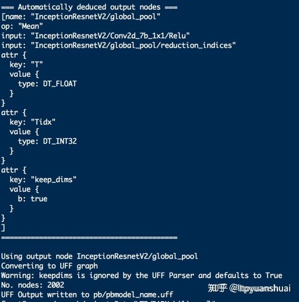
如转换成功会输出如下信息，包含图中总结点的个数以及推断出的输入输出节点的信息

（3）tensorRT c++ API 部署模型

使用 tensorRT 部署生成好的 uff 模型需要先讲 uff 中保存的模型权值以及网络结构导入进来，然后执行优化算法生成对应的 inference engine。具体代码如下，首先需要定义一个 IBuilder* builder，一个用来解析 uff 文件的 parser 以及 builder 创建的 network，parser 会将 uff 文件中的模型参数和网络结构解析出来存到 network，解析前要预先告诉 parser 网络输入输出输出的节点。解析后 builder 就能根据 network 中定义的网络结构创建 engine。在创建 engine 前会需要指定最大的 batchsize 大小，之后使用 engine 时输入的 batchsize 不能超过这个数值否则就会出错。推断时如果 batchsize 和设定最大值一样时效率最高。举个例子，如果设定最大 batchsize 为 10，实际推理输入一个 batch 10 张图的时候平均每张推断时间是 4ms 的话，输入一个 batch 少于 10 张图的时候平均每张图推断时间会高于 4ms。

IBuilder* builder = createInferBuilder(gLogger.getTRTLogger());
auto parser = createUffParser();
parser->registerInput(inputtensor_name, Dims3(INPUT_C, INPUT_H, INPUT_W), UffInputOrder::kNCHW);
parser->registerOutput(outputtensor_name);
    INetworkDefinition* network = builder->createNetwork();
    if (!parser->parse(uffFile, *network, nvinfer1::DataType::kFLOAT))
    {
        gLogError << "Failure while parsing UFF file" << std::endl;
        return nullptr;
    }  
    builder->setMaxBatchSize(maxBatchSize);
    builder->setMaxWorkspaceSize(MAX_WORKSPACE);
    ICudaEngine* engine = builder->buildCudaEngine(*network);
    if (!engine)
    {
        gLogError << "Unable to create engine" << std::endl;
        return nullptr;
    }

生成 engine 之后就可以进行推断了，执行推断时需要有一个上下文执行上下文 IExecutionContext* context，可以通过 engine->createExecutionContext () 获得。执行推断的核心代码是

1	context->execute(batchSize, &buffers[0]);

其中 buffer 是一个 void * 数组对应的是模型输入输出 tensor 的设备地址，通过 cudaMalloc 开辟输入输出所需要的设备空间（显存）将对应指针存到 buffer 数组中，在执行 execute 操作前通过 cudaMemcpy 把输入数据（输入图像）拷贝到对应输入的设备空间，执行 execute 之后还是通过 cudaMemcpy 把输出的结果从设备上拷贝出来。

更为详细的例程可以参考 TensorRT 官方的 samples 中的 sampleUffMNIST 代码

（4）加速比情况

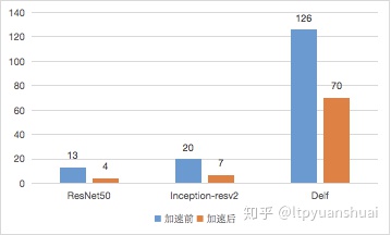
实际工程中我在 Tesla M40 上用 tensorRT 来加速过 Resnet-50，Inception-resnet-v2，谷歌图像检索模型 Delf（DEep Local Features），加速前后单张图推断用时比较如下图（单位 ms）

4> Caffe 模型 tensorRT 部署教程

相比与 tensorflow 模型 caffe 模型的转换更加简单，不需要有 tensorflow 模型转 uff 模型这类的操作，tensorRT 能够直接解析 prototxt 和 caffemodel 文件获取模型的网络结构和权重。具体解析流程和上文描述的一致，不同的是 caffe 模型的 parser 不需要预先指定输入层，这是因为 prototxt 已经进行了输入层的定义，parser 能够自动解析出输入，另外 caffeparser 解析网络后返回一个 IBlobNameToTensor *blobNameToTensor 记录了网络中 tensor 和 pototxt 中名字的对应关系，在解析之后就需要通过这个对应关系，按照输出 tensor 的名字列表 outputs 依次找到对应的 tensor 并通过 network->markOutput 函数将其标记为输出，之后就可以生成 engine 了。

IBuilder* builder = createInferBuilder(gLogger);
    INetworkDefinition* network = builder->createNetwork();
    ICaffeParser* parser = createCaffeParser();
    DataType modelDataType = DataType::kFLOAT;
    const IBlobNameToTensor *blobNameToTensor =	parser->parse(deployFile.c_str(),
                                                              modelFile.c_str(),
                                                              *network,
                                                              modelDataType);
    assert(blobNameToTensor != nullptr);
    for (auto& s : outputs) network->markOutput(*blobNameToTensor->find(s.c_str()));
 
    builder->setMaxBatchSize(maxBatchSize);
    builder->setMaxWorkspaceSize(1 << 30);
    engine = builder->buildCudaEngine(*network);

生成 engine 后执行的方式和上一节描述的一致，详细的例程可以参考 SampleMNIST

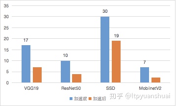
（1）加速比情况

实际工程中我在 Tesla M40 上用 tensorRT 加速过 caffe 的 VGG19，SSD 速度变为 1.6 倍，ResNet50，MobileNetV2 加速前后单张图推断用时比较如下图（单位 ms）

5> 为 tensorRT 添加自定义层

tensorRT 目前只支持一些非常常见的操作，有很多操作它并不支持比如上采样 Upsample 操作，这时候就需要我们自行将其编写为 tensorRT 的插件层，从而使得这些不能支持的操作能在 tensorRT 中使用。以定义 Upsample 层为例，我们首先要定义一个继承自 tensorRT 插件基类的 Upsample 类

1	class Upsample: public IPluginExt

然后要实现该类的一些必要方法，首先是 2 个构造函数，一个是传参数构建，另一个是从序列化后的比特流构建。

 Upsample(int scale = 2) : mScale(scale) {
        assert(mScale > 0);
    }
//定义上采样倍数
 Upsmaple(const void *data, size_t length) {
        const char *d = reinterpret_cast<const char *>(data), *a = d;
        mScale = read<int>(d);
        mDtype = read<DataType>(d);
        mCHW = read<DimsCHW>(d);
        assert(mScale > 0);
        assert(d == a + length);
    }
~Upsample()
    {

    }

一些定义层输出信息的方法

   int getNbOutputs() const override {
        return 1;
    }
//模型的输出个数
    Dims getOutputDimensions(int index, const Dims *inputs, int nbInputDims) override {
       // std::cout << "Get ouputdims!!!" << std::endl;
        assert(nbInputDims == 1);
        assert(inputs[0].nbDims == 3);
        return DimsCHW(inputs[0].d[0], inputs[0].d[1] * mScale, inputs[0].d[2] * mScale);
    }
//获取模型输出的形状

根据输入的形状个数以及采用的数据类型检查合法性以及配置层参数的方法

    bool supportsFormat(DataType type, PluginFormat format) const override {
        return (type == DataType::kFLOAT || type == DataType::kHALF || type == DataType::kINT8)
               && format == PluginFormat::kNCHW;
    }
//检查层是否支持当前的数据类型和格式
    void configureWithFormat(const Dims *inputDims, int nbInputs, const Dims *outputDims, int nbOutputs,
                             DataType type, PluginFormat format, int maxBatchSize) override
       {
         mDtype = type;
         mCHW.c() = inputDims[0].d[0];
         mCHW.h() = inputDims[0].d[1];
         mCHW.w() = inputDims[0].d[2];
        }
//配置层的参数

层的序列化方法

 size_t getSerializationSize() override {
        return sizeof(mScale) + sizeof(mDtype) + sizeof(mCHW);
    }
//输出序列化层所需的长度
    void serialize(void *buffer) override {
        char *d = reinterpret_cast<char *>(buffer), *a = d;
        write(d, mScale);
        write(d, mDtype);
        write(d, mCHW);
        assert(d == a + getSerializationSize());
    }
//将层参数序列化为比特流

层的运算方法

 size_t getWorkspaceSize(int maxBatchSize) const override {
        return 0;
    }
//层运算需要的临时工作空间大小
 int enqueue(int batchSize, const void *const *inputs, void **outputs, void *workspace,
                cudaStream_t stream) override;
//层执行计算的具体操作

在 enqueue 中我们调用编写好的 cuda kenerl 来进行 Upsample 的计算

完成了 Upsample 类的定义，我们就可以直接在网络中添加我们编写的插件了，通过如下语句我们就定义一个上采样 2 倍的上采样层。addPluginExt 的第一个输入是 ITensor** 类别，这是为了支持多输出的情况，第二个参数就是输入个数，第三个参数就是需要创建的插件类对象。

1 2	Upsample up(2)； auto upsamplelayer=network->addPluginExt(inputtensot,1,up)

6> 为 CaffeParser 添加自定义层支持

对于我们自定义的层如果写到了 caffe prototxt 中，在部署模型时调用 caffeparser 来解析就会报错。

还是以 Upsample 为例，如果在 prototxt 中有下面这段来添加了一个 upsample 的层

layer {
  name: "upsample0"
  type: "Upsample"
  bottom: "ReLU11"
  top: "Upsample1"
}

这时再调用

const IBlobNameToTensor *blobNameToTensor =	parser->parse(deployFile.c_str(),
                                                              modelFile.c_str(),
                                                              *network,
                                                              modelDataType);

就会出现错误

之前我们已经编写了 Upsample 的插件，怎么让 tensorRT 的 caffe parser 识别出 prototxt 中的 upsample 层自动构建我们自己编写的插件呢？这时我们就需要定义一个插件工程类继承基类 nvinfer1::IPluginFactory, nvcaffeparser1::IPluginFactoryExt。

1	class PluginFactory : public nvinfer1::IPluginFactory, public nvcaffeparser1::IPluginFactoryExt

其中必须要的实现的方法有判断一个层是否是 plugin 的方法，输入的参数就是 prototxt 中 layer 的 name，通过 name 来判断一个层是否注册为插件

bool isPlugin(const char *name) override {
        return isPluginExt(name);
    }
 
bool isPluginExt(const char *name) override {
 
        char *aa = new char[6];
        memcpy(aa, name, 5);
        aa[5] = 0;
        int res = !strcmp(aa, "upsam");
        return res;
}
//判断层名字是否是upsample层的名字

根据名字创建插件的方法，有两中方式一个是由权重构建，另一个是由序列化后的比特流创建，对应了插件的两种构造函数，Upsample 没有权重，对于其他有权重的插件就能够用传入的 weights 初始化层。mplugin 是一个 vector 用来存储所有创建的插件层。

IPlugin *createPlugin(const char *layerName, const nvinfer1::Weights *weights, int nbWeights) override {
        assert(isPlugin(layerName));
        mPlugin.push_back(std::unique_ptr<Upsample>(new Upsample(2)));
        return mPlugin[mPlugin.size() - 1].get();
    }
IPlugin *createPlugin(const char *layerName, const void *serialData, size_t serialLength) override {
        assert(isPlugin(layerName));
        return new Upsample(serialData, serialLength);
    }
 std::vector <std::unique_ptr<Upsample>> mPlugin;

最后需要定义一个 destroy 方法来释放所有创建的插件层。

 void destroyPlugin() {
        for (unsigned int i = 0; i < mPlugin.size(); i++) {
            mPlugin[i].reset();
        }
}

对于 prototxt 存在多个多种插件的情况，可以在 isPlugin，createPlugin 方法中添加新的条件分支，根据层的名字创建对应的插件层。

实现了 PluginFactory 之后在调用 caffeparser 的时候需要设置使用它，在调用 parser->parser 之前加入如下代码

1 2	PluginFactory pluginFactory; parser->setPluginFactoryExt(&pluginFactory);

就可以设置 parser 按照 pluginFactory 里面定义的规则来创建插件层，这样之前出现的不能解析 Upsample 层的错误就不会再出现了。

官方添加插件层的样例 samplePlugin 可以作为参考

7> 心得体会（踩坑记录）

转 tensorflow 模型时，生成 pb 模型、转换 uff 模型以及调用 uffparser 时 register Input，output，这三个过程中输入输出节点的名字一定要注意保持一致，否则最终在 parser 进行解析时会出现错误，找不到输入输出节点。
除了本文中列举的 pluginExt，tensorRT 中插件基类还有 IPlugin，IPluginV2，继承这些基类所需要实现的类方法有细微区别，具体情况可自行查看 tensorRT 安装文件夹下的 include/NvInfer.h 文件。同时添加自己写的层到网络时的函数有 addPlugin，addPluginExt，addPluginV2 这几种和 IPlugin，IPluginExt，IPluginV2 一一对应，不能够混用，否则有些默认调用的类方法不会调用的，比如用 addPlugin 添加的 PluginExt 层是不会调用 configureWithFormat 方法的，因为 IPlugin 类没有该方法。同样的在还有 caffeparser 的 setPluginFactory 和 setPluginFactoryExt 也是不能混用的。
运行程序出现 cuda failure 一般情况下是由于将内存数据拷贝到磁盘时出现了非法内存访问，注意检查 buffer 开辟的空间大小和拷贝过去数据的大小是否一致.
有一些操作在 tensorRT 中不支持但是可以通过一些支持的操作进行组合替代，比如，这样可以省去一些编写自定义层的时间。
tensorflow 中的 flatten 操作默认时 keepdims=False 的，但是在转化 uff 文时会默认按照 keepdims=True 转换，因此在 tensorflow 中对 flatten 后的向量进行 transpose、expanddims 等等操作，在转换到 uff 后用 tensorRT 解析时容易出现错误，比如 “Order size is not matching the number dimensions of TensorRT” 。最好设置 tensorflow 的 reduce，flatten 操作的 keepdims=True，保持层的输出始终为 4 维形式，能够有效避免转到 tensorRT 时出现各种奇怪的错误。
tensorRT 中的 slice 层存在一定问题，我用 network->addSlice 给网络添加 slice 层后，在执行 buildengine 这一步时就会出错 nvinfer1::builder::checkSanity (const nvinfer1::builder::Graph&): Assertion `tensors.size () == g.tensors.size ()’ failed.，构建网络时最好避开使用 slice 层，或者自己实现自定层来执行 slice 操作。
tensorRT 的 github 中有着部分的开源代码以及丰富的示例代码，多多学习能够帮助更快的掌握 tensorRT 的使用

最后更新： 2022年03月03日 23:18

原始链接： https://leezhao415.github.io/2022/03/03/%E3%80%90%E7%B2%BE%E5%8D%8E%E3%80%91%E6%A8%A1%E5%9E%8B%E9%83%A8%E7%BD%B2%E5%AE%9E%E4%BE%8B%EF%BC%88OpenVINO%E3%80%81TensorRT%EF%BC%89/

赏

LeeZhao's Blog

且听风吟，御剑于心！